Reinforcement Learning#
Introduction#
Reinforcement Learning is a branch of machine learning that focuses on how agents should act in an environment to maximize a notion of cumulative reward. Unlike supervised learning, where algorithms are trained on labeled examples, RL learns from a trial-and-error process based on the environment’s responses to its actions.
Differences between RL and other learning methods:
Supervised learning: Algorithms learn from labeled examples, trying to predict label based on the training set;
Unsupervised learning: Algorithms try to find patterns in the data, without any labels;
Reinforcement learning: Agent learns to make decision through rewards (or punishments) received from its actions.
Key elements:
Agent:
Definition: The agent is the entity that makes decisions and learns through interaction with the environment. In RL, the agent chooses actions to take based on its current policy.
Role in RL: The agent is at the center of learning in RL. Its goal is to learn the best possible policy, that is, a map from states to actions, to maximize the total reward collected over time.
Enviroment:
Definition: Environment represents the context or world in which the agent operates. It includes anything that the agent can interact with but does not have direct control over;
Interaction with the agent: The environment responds to the agent’s actions and presents new states and rewards to the agent. The nature of the environment can vary from simple and static to complex and dynamic.
State:
Definition: A state is a configuration or representation of the environment at a given time. States provide the information the agent needs to make decisions.
Importance: The quality and quantity of information available in states can significantly influence the effectiveness of agent learning.
Action:
Definition: Actions are the various behaviors or moves that the agent can perform. The set of all available actions is known as the action space.
Action-Stata dynamics: Every action taken by the agent affects the state of the environment. The relationship between actions and their consequence on states is fundamental to the agent’s decision making.
Reward:
Definnition: A reward is immediate feedback provided to the agent by the environment as a consequence of his or her actions. Rewards can be positive (to encourage certain actions) or negative (to discourage certain actions).
Role in learning: Rewards are the main guide for the agent in the learning process. The agent’s goal is to maximize the sum of rewards over time, often referred to as return.
Policy:
Definition: A policy is a strategy adopted by the agent, a kind of rule or algorithm that decides what action to take based on the current state.
Types: Policies can be deterministic or stochastic. A deterministic policy always provides the same action for a given state, while a stochastic policy selects actions according to a probability distribution.
Evaluation functions:
Goal: These functions help the agent evaluate the effectiveness of his or her actions and policies.
Types:
Value function: Estimates the expected return from a state following a given policy.
Q-Value function: also known as Action-Value function. Estimates the expected return for a state-action pair.
Model:
Description: A model is an internal representation of the environment that the agent uses to predict how the environment will respond to its actions.
Model-based vs model-free RL: In model-based RL, the agent uses an explicit model of the environment to plan its actions. In model-free RL, the agent learns directly from interactions with the environment without an explicit model.
Theoretical concepts#
1. Markov Decision Process#
The Markov Decision Process (MDP) is a fundamental mathematical framework in the field of Reinforcement Learning. It provides a formalization for decision-making in uncertain and dynamic situations. An MDP is characterized by a set of states, a set of actions, transition probabilities and reward functions.
Key MDP elements:
States: A set of states \(S\) represents all the possible configurations the environment can be in.
Actions: A set of actions \(A\) that the agent can take. The set of available actions may depend on the current state.
Transition probability: A transaction function \(P(s_{t+1} | s_t, a_t)\) which defines the probability of transition to the state \(s_{t+1}\) given the current state \(s_t\) and action \(a_t\).
Reward: A reward function \(R(s_t, a_t, s_{t+1})\) which assigns a reward (or a punishment) to the agent for the transition from state \(s_t\) to state \(s_{t+1}\) after taking action \(a_t\).
The fundamental property of an MDP is the “Markov property,” which states that the future is independent of the past given the present. This means that the transition probability and reward depend only on the current state and the action taken, not on the history of previous actions or states.
2. Reward and evaluation function#
In the context of Reinforcement Learning, the reward and evaluation function are central concepts that guide agent learning and decision-making. This chapter explores the nature of these components and their role in RL.
Reward:
Definition: A reward is a scalar value that represents the immediate feedback provided to the agent by the environment as a consequence of his or her actions. Rewards can be positive (to encourage certain actions) or negative (to discourage certain actions).
Role in learning: Rewards are the main guide for the agent in the learning process. The agent’s goal is to maximize the sum of rewards over time, often referred to as return.
Evaluation function:
Value function: The value function, denoted as \(V(s)\), estimates the expected total return from a states following a given policy. It provides a measure of the goodness-of-fit of a state.
Q-value function: The Q-value function, or action-value function, denoted as \(Q(s, a)\), evaluates the action \(a\) in the state \(s\). It estimates the expected return following the action \(a\) in the state \(s\) and then adhering to a specific policy.
3. Common RL algorithms#
Q-learning is a model-free learning method that seeks to learn an optimal policy independently of the agent’s current action. The algorithm iteratively updates the Q-value estimates for each state-action pair using the Q-learning update formula, based on the reward received and the maximum Q-value of the next state. Q-learning is widely used for problems with discrete state and action spaces and is well suited to situations with uncertain environmental dynamics.
SARSA is a model-based differential time learning (TD) algorithm. Unlike Q-learning, SARSA updates its Q-values based on the agent’s current policy (on-policy). The update considers the current transition and the next action the agent intends to perform. SARSA is useful in environments where risk assessment and safety considerations are important because it takes into account the actual path the agent plans to follow.
Some remarks:
Exploration vs. exploitation: A key aspect in RL is the balance between exploration (trying new actions) and exploitation (using acquired knowledge). RL algorithms must effectively manage this balance;
Scalability and complexity: the scalability of algorithms in environments with large state and action spaces is a significant challenge. Methods such as deep learning have been integrated into RL to address this challenge.
Use of RL in finance#
In trading, RL can be used to develop automated strategies that decide when to buy, sell, or hold a stock or cryptocurrency. Financial markets are complex, noisy, and nonstationary, making trading an ideal challenge for RL, which can adapt to such dynamic conditions.
Challenges:
Financial data are often noisy and exhibit nonstationarity, which can lead to overfitting and inconsistent model performance.
Markets change rapidly, and what has worked in the past may no longer be valid, requiring the model to continually adapt.
Pros of using RL:
Automation and Scalability: The RL can automate trading decisions and operate on a large scale, analyzing huge amounts of data more efficiently than human analysis.
Adaptability: RL models can dynamically adapt to changes in the market, continuously learning from new data.
High Performance Potential: When configured well, RL models can potentially outperform traditional strategies and human traders, especially in highly volatile markets.
Common approaches:
Deep reinforcement learning: The use of deep neural networks to handle the complexity of market data and capture nonlinear relationships.
Optimized exploration strategies: Development of exploration methods that balance between learning from historical market situations and exploring new trading strategies.
Practical implementation#
Introduction to Financial Market Simulation with Gym-MTSim#
In this section of our Jupyter Notebook, we explore the world of financial market simulation using the gym_mtsim library, an extension of OpenAI’s Gym. The Gym library provides a standardized interface for reinforcement learning (RL) tasks, and gym_mtsim specifically caters to financial market simulations, offering a unique and practical approach for testing and developing financial strategies in a controlled, simulated environment.
The code snippet provided initializes various environments that simulate different financial markets and trading scenarios. Each environment corresponds to a unique market type or strategy:
Forex Markets (Hedged and Unhedged):
forex-hedge-v0simulates a foreign exchange (Forex) market with a hedging strategy.forex-unhedge-v0represents the Forex market without a hedging strategy.
Stock Markets (Hedged and Unhedged):
stocks-hedge-v0sets up a simulated environment for stock market trading with a hedging strategy.stocks-unhedge-v0offers a simulation of stock market trading without the use of hedging.
Cryptocurrency Markets (Hedged and Unhedged):
crypto-hedge-v0is tailored for cryptocurrency market simulations implementing hedging strategies.crypto-unhedge-v0provides a crypto market environment without hedging.
Mixed Asset Markets (Hedged and Unhedged):
mixed-hedge-v0creates a diverse market environment with multiple asset types, using hedging strategies.mixed-unhedge-v0simulates a mixed asset market without the use of hedging strategies.
Each of these environments can be used to train and evaluate RL models, providing insights into different trading strategies and market behaviors. This approach is invaluable for researchers and practitioners in the field of quantitative finance, offering a risk-free platform to experiment and refine trading algorithms.
import plotly.offline as pyo
pyo.init_notebook_mode(connected=True)
import warnings
warnings.filterwarnings('ignore')
import gym
import gym_mtsim

env = gym.make('forex-hedge-v0')
# env = gym.make('stocks-hedge-v0')
# env = gym.make('crypto-hedge-v0')
# env = gym.make('mixed-hedge-v0')

# env = gym.make('forex-unhedge-v0')
# env = gym.make('stocks-unhedge-v0')
# env = gym.make('crypto-unhedge-v0')
# env = gym.make('mixed-unhedge-v0')
Setting Up a Reinforcement Learning Environment for Forex Trading with Gym-MTSim#
In this section of our Jupyter Notebook, we delve into setting up a more advanced financial market simulation environment using gym_mtsim. This setup is specifically tailored for reinforcement learning (RL) applications in Forex trading. Our focus is to demonstrate how RL can be applied in the complex and dynamic world of foreign exchange markets.
The provided code snippet establishes a simulated trading environment, which is a critical step for training RL agents. Here’s a detailed breakdown of the components and their roles:
Importing Necessary Libraries and Modules:
pytz: For timezone operations, crucial in time-sensitive financial markets.datetime,timedelta: For handling date and time, essential for simulating real-time market scenarios.numpy: A fundamental package for scientific computing, used here for statistical operations.gym_mtsim: The core library for creating the Forex market simulation environment.MtEnv,MtSimulator,FOREX_DATA_PATH: Specific classes and constants fromgym_mtsimused for setting up the environment.
Initializing the Market Simulator (
MtSimulator):Currency and Balance: The simulation uses USD as the base unit with an initial balance of $10,000.
Leverage and Risk Management: A leverage of 100x is set, along with a stop-out level at 20% to manage risk.
Hedging: The simulator is configured to allow hedging strategies.
Market Data: The
symbols_filenameparameter points to the Forex market data source.
Creating the Trading Environment (
MtEnv):Trading Symbols: We focus on three currency pairs: GBPCAD, EURUSD, and USDJPY.
Window Size: A window size of 10 is set, determining how much past data is visible to the agent at any point.
Thresholds for Holding and Closing Positions: Both set to 0.5, dictating the agent’s decision-making criteria.
Trading Fees: Dynamically calculated based on the currency pair, introducing a realistic aspect of cost in trading.
Order Limits and Parallel Processing: Each symbol can have up to 2 orders, and the environment supports multiprocessing with 2 processes.
This setup provides a rich and realistic environment for training RL agents. The agents can learn and adapt their trading strategies based on historical data, market conditions, and transaction costs. The complexity of this environment, with its multiple currency pairs and dynamic fee structure, offers a challenging yet rewarding platform for exploring the capabilities of RL in Forex trading.
In the following parts of the notebook, we will introduce the RL concepts and algorithms, and demonstrate how they can be trained within this environment to make informed trading decisions. This practical application not only showcases the power of RL in financial decision-making but also provides a hands-on experience in applying advanced AI techniques in the domain of quantitative finance.
import pytz
from datetime import datetime, timedelta
import numpy as np
from gym_mtsim import MtEnv, MtSimulator, FOREX_DATA_PATH


sim = MtSimulator(
    unit='USD',
    balance=10000.,
    leverage=100.,
    stop_out_level=0.2,
    hedge=True,
    symbols_filename=FOREX_DATA_PATH
)

env = MtEnv(
    original_simulator=sim,
    trading_symbols=['GBPCAD', 'EURUSD', 'USDJPY'],
    window_size=10,
    # time_points=[desired time points ...],
    hold_threshold=0.5,
    close_threshold=0.5,
    fee=lambda symbol: {
        'GBPCAD': max(0., np.random.normal(0.0007, 0.00005)),
        'EURUSD': max(0., np.random.normal(0.0002, 0.00003)),
        'USDJPY': max(0., np.random.normal(0.02, 0.003)),
    }[symbol],
    symbol_max_orders=2,
    multiprocessing_processes=2
)
for symbol in env.prices:
    print(f"prices[{symbol}].shape:", env.prices[symbol].shape)

print("signal_features.shape:", env.signal_features.shape)
print("features_shape:", env.features_shape)
prices[GBPCAD].shape: (88, 2)
prices[EURUSD].shape: (88, 2)
prices[USDJPY].shape: (88, 2)
signal_features.shape: (88, 6)
features_shape: (10, 6)
In this section of our Jupyter Notebook, we demonstrate a basic loop for simulating a trading environment using the setup we previously created with gym_mtsim. This loop is fundamental for training reinforcement learning (RL) agents, where they interact with the environment, receive feedback (rewards), and adjust their actions accordingly.
Here’s a detailed explanation of the code snippet and its role in the RL context:
Environment Reset (
env.reset()):This initializes or resets the environment to a starting state. It’s akin to starting a new trading day or session, where the RL agent begins with a clean slate.
The
resetmethod returns an initial observation, providing the agent with the current state of the market.
Trading Loop:
The
while True:loop represents the continuous process of trading in a market. Each iteration of the loop is analogous to a single step or action taken by the RL agent in the environment.
Sampling an Action (
env.action_space.sample()):At each step, an action is selected randomly from the action space. In a more sophisticated RL setup, this is where the agent’s policy or decision-making logic would determine the action based on the current state (observation).
The action could involve buying, selling, holding, or other trading actions specific to the environment’s design.
Taking a Step (
env.step(action)):The
stepmethod advances the environment by one time step using the chosen action. It returns several important pieces of information:observation: The new state of the market after the action is taken.reward: The immediate reward received after taking the action, which is crucial for RL as it guides the agent’s learning process.done: A boolean indicating whether the episode (trading session) has ended (e.g., due to bankruptcy, reaching a time limit, etc.).info: A dictionary containing supplementary information such as balance, equity, margin levels, etc.
Handling the End of an Episode (
if done:):If
doneis True, it signals the end of the trading episode. This can trigger the agent to evaluate its performance and learn from the episode.The code then prints out important financial metrics from the
infodictionary:balance,equity,margin,free_margin, andmargin_levelprovide insights into the financial status at the end of the episode.step_rewardgives the reward obtained in the final step, which could be used for further analysis or learning.
This loop forms the core of an RL training process in financial market simulation. In a complete RL application, the agent would not randomly select actions but instead follow a strategy based on its learning and the observed states. The
feedback from the environment in terms of rewards and state transitions guides the agent to refine its strategy over time, aiming to maximize cumulative rewards, which in the context of trading, could align with maximizing profit or minimizing risk.
In subsequent sections of our notebook, we will explore how to replace the random action selection with a decision-making policy driven by RL algorithms. We will also look into how the agent learns from the environment’s feedback, adjusts its trading strategy, and improves its performance over successive trading episodes. This iterative learning process is at the heart of applying RL in financial trading simulations, providing valuable insights and practical skills in leveraging AI for quantitative finance.
observation = env.reset()

while True:
    action = env.action_space.sample()
    observation, reward, done, info = env.step(action)
    if done:
        print(
            f"balance: {info['balance']}, equity: {info['equity']}, margin: {info['margin']}\n"
            f"free_margin: {info['free_margin']}, margin_level: {info['margin_level']}\n"
            f"step_reward: {info['step_reward']}"
        )
        break
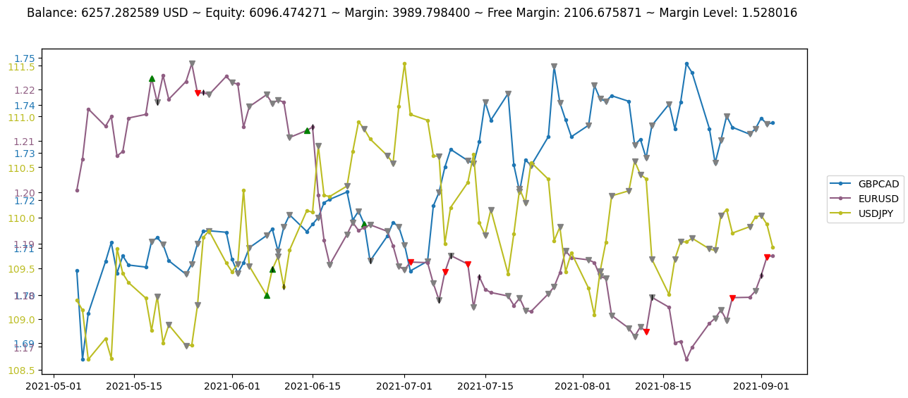
balance: 6257.282588625643, equity: 6096.474270944401, margin: 3989.7984
free_margin: 2106.6758709444007, margin_level: 1.5280156187702116
step_reward: -160.80831768124244
Custom accuracy#
In the realm of stock trading using reinforcement learning, the tradtional concept of accuracy, as used in supervised learning, does not directly apply. In supervised learning, accuracy is typically a measure of how many predictions a model got right. However, in stock trading, success is not just about the requency of correct predictions. but also about the quality and profitability of the trades made. Therefore, we need a different approach to measure the performance of an RL model in sotck trading. This is where the concept of custom accuracy, specifically designed for trading, comes into play.
Custom accuracy: Profitable Trades Ratio#
The Profitable Trades Ratio is straightforward yet effective metric for assessing the performance of a stock trading RL model. This metric focuses on the proportion of trades that resulted in a profit, regardless of the size of the profit
Definition Profitable Trades Ration is defined as the ratio of the number of profitable trades to the total number of trades made by the model.
Advantages
Simplicity: The metric is straightforward to calculate and understand.
Direct Relevance: It directly relates to the fundamental goal of trading, which is to make profitable trades.
Limitations
Does not reflect magnitude: It doesn’t account for the size of the profit or loss in each trade.
Risk ignorance: It does not consider the risk involved in achieving the profits.
May not represent overall performance: A few large losses could offset many small wins, which this metric would not reveal.
def calculate_profitable_trades_ratio(trades):
    profitable_trades = sum(1 for index, trade in trades.iterrows() if trade['Exit Price'] > trade['Entry Price'])
    total_trades = len(trades)
    return profitable_trades / total_trades if total_trades > 0 else 0
Printing the results
state = env.render()

custom_accuracy = calculate_profitable_trades_ratio(state['orders'])

print(f"profitable trades ratio: {custom_accuracy}\n")
state['orders']
profitable trades ratio: 0.5833333333333334
| Id | Symbol | Type | Volume | Entry Time | Entry Price | Exit Time | Exit Price | Profit | Margin | Fee | Closed | |
|---|---|---|---|---|---|---|---|---|---|---|---|---|
| 0 | 12 | EURUSD | Sell | 3.36 | 2021-09-02 00:00:00+00:00 | 1.18744 | 2021-09-03 00:00:00+00:00 | 1.18772 | -160.808318 | 3989.798400 | 0.000199 | False |
| 1 | 11 | EURUSD | Sell | 6.16 | 2021-08-27 00:00:00+00:00 | 1.17955 | 2021-09-01 00:00:00+00:00 | 1.18384 | -2787.425464 | 7266.028000 | 0.000235 | True |
| 2 | 10 | EURUSD | Sell | 0.21 | 2021-08-12 00:00:00+00:00 | 1.17296 | 2021-08-13 00:00:00+00:00 | 1.17962 | -145.195089 | 246.321600 | 0.000254 | True |
| 3 | 9 | EURUSD | Sell | 1.85 | 2021-07-12 00:00:00+00:00 | 1.18606 | 2021-07-14 00:00:00+00:00 | 1.18358 | 432.181706 | 2194.211000 | 0.000144 | True |
| 4 | 8 | EURUSD | Sell | 4.22 | 2021-07-08 00:00:00+00:00 | 1.18449 | 2021-07-09 00:00:00+00:00 | 1.18774 | -1471.050459 | 4998.547800 | 0.000236 | True |
| 5 | 7 | EURUSD | Sell | 2.75 | 2021-07-02 00:00:00+00:00 | 1.18646 | 2021-07-07 00:00:00+00:00 | 1.17903 | 1989.132017 | 3262.765000 | 0.000197 | True |
| 6 | 6 | GBPCAD | Buy | 1.03 | 2021-06-24 00:00:00+00:00 | 1.71493 | 2021-06-25 00:00:00+00:00 | 1.70721 | -707.728647 | 1433.457415 | 0.000730 | True |
| 7 | 5 | EURUSD | Buy | 4.01 | 2021-06-14 00:00:00+00:00 | 1.21200 | 2021-06-15 00:00:00+00:00 | 1.21264 | 204.656503 | 4860.120000 | 0.000130 | True |
| 8 | 4 | USDJPY | Buy | 2.49 | 2021-06-08 00:00:00+00:00 | 109.49200 | 2021-06-10 00:00:00+00:00 | 109.31900 | -443.671597 | 2490.000000 | 0.021786 | True |
| 9 | 3 | USDJPY | Buy | 5.98 | 2021-06-07 00:00:00+00:00 | 109.23800 | 2021-06-08 00:00:00+00:00 | 109.49200 | 1292.026249 | 5980.000000 | 0.017434 | True |
| 10 | 2 | EURUSD | Sell | 1.99 | 2021-05-26 00:00:00+00:00 | 1.21922 | 2021-05-27 00:00:00+00:00 | 1.21934 | -68.261126 | 2426.247800 | 0.000223 | True |
| 11 | 1 | EURUSD | Buy | 4.10 | 2021-05-18 00:00:00+00:00 | 1.22219 | 2021-05-19 00:00:00+00:00 | 1.21744 | -2037.381504 | 5010.979000 | 0.000219 | True |
Render in simple_figure mode
Each symbol is illustrated in a different color
The green/red triangle show successful buy/sell actions
The grey triangles indicate that the buy/sell actions encountered and error
The black vertical bars specify close actions
env.render('simple_figure')
Render in advanced_mode figure
Clicking on a symbol name will hide/show its plot
Hovering over points and markers will display their details
The size of the triangles indicates their relative volume
env.render('advanced_figure', time_format='%Y-%m-%d')